Fist-Steps
This chapter offers a quick overview of the main package capabilities: To read a sounding from a txt file and create a quick SkewT diagram.
Fist steps using SkewTplus
From now on, it’s assumed that the package is installed and the current working directory is the examples one, included in this package.
To read a sounding from a txt file and create a quick plot using the default parameters we only have to do:
from SkewTplus.sounding import Sounding

#Load the sounding data
mySounding = sounding("./exampleSounding.txt")
mySounding.quickPlot()
The resulting plot will look like this:
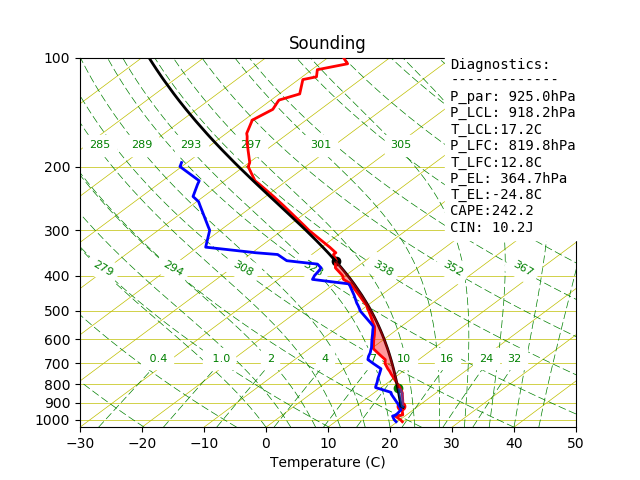
Now we can do the same thing, but with more control over the Figure:
# Import the new figure class
from SkewTplus.skewT import figure

from SkewTplus.sounding import sounding


#Load the sounding data
mySounding = sounding("./exampleSounding.txt")

# Create a Figure Manager
mySkewT_Figure = figure()

# Add an Skew-T axes to the Figure
mySkewT_Axes = mySkewT_Figure.add_subplot(111, projection='skewx')


# Extract the data from the Sounding
pressure = mySounding.soundingdata['pres']
temperature =  mySounding.soundingdata['temp']
dewPointTemperature = mySounding.soundingdata['dwpt']

# Add a profile to the Skew-T diagram
#  method=0 -> Most unstable parcel
#  diagnostics -> add a text box in the Figure with the parcel analysis results
mySkewT_Axes.addProfile(pressure,temperature, dewPointTemperature ,
                            hPa=True, celsius=True, method=0, diagnostics=True)

# Show the figure
mySkewT_Figure.show()

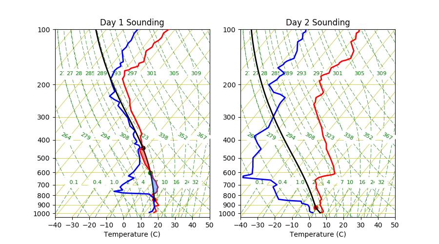
Lets now complicate the things a little bit and show one of the new capabilities of the package. Let suppose that we want to compare two soundings, with the parcel analysis, and plot them side to side:
#Load the sounding data
mySounding1 = sounding("./bna_day1.txt")
mySounding2 = sounding("./bna_day2.txt")

# Create a Figure Manager with a suitable size for both plots
mySkewT_Figure = figure(figsize=(9,5))

# Now we want to create two axes side to side

# Add the first Skew-T axes to the Figure
mySkewT_Axes1 = mySkewT_Figure.add_subplot(121, projection='skewx',tmin=-40)


# Extract the data from the Sounding
pressure = mySounding1['pres']
temperature =  mySounding1['temp']
dewPointTemperature = mySounding1['dwpt']

# Add a profile to the Skew-T diagram
mySkewT_Axes1.addProfile(pressure,temperature, dewPointTemperature ,
                        hPa=True, celsius=True, method=0, diagnostics=False)


mySkewT_Axes1.set_title("Day 1 Sounding")

# Add the second Skew-T axes to the Figure
mySkewT_Axes2 = mySkewT_Figure.add_subplot(122, projection='skewx',tmin=-40)

# Extract the data from the Sounding
pressure = mySounding2['pres']
temperature =  mySounding2['temp']
dewPointTemperature = mySounding2['dwpt']

# Add a profile to the Skew-T diagram
mySkewT_Axes2.addProfile(pressure,temperature, dewPointTemperature ,
                        hPa=True, celsius=True, method=0, diagnostics=False)

mySkewT_Axes2.set_title("Day 2 Sounding")

# Show the figure
mySkewT_Figure.show_plot()
The different sounding sources supported to initialize the
sounding class are described
in greater detail in the next chapter:
Sounding Initialization