Parcel Analysis

The SkewTplus package comes with the SkewTplus.thermodynamics module that allows the following computations for a parcel:

• SkewTplus.thermodynamics.parcelAnalysis()
• SkewTplus.thermodynamics.liftParcel()
• SkewTplus.thermodynamics.moistAscent()
• SkewTplus.thermodynamics.getLCL()

parcelAnalysis Function

The SkewTplus.thermodynamics.parcelAnalysis() function not only supports computations on 1D vertical soundings, also it allows to do the analysis in a 3D domain (height,latitude or y ,longitude or x) or 4D=(3D + time) ones (time,height,latitude or y ,longitude or x].

Below is simple example of how to perform a parcel analysis, print the results and then plot the parcel trajectory. For this example you need netCDF4 and Basemap packages installed:

from SkewTplus.skewT import figure
from SkewTplus.sounding import sounding
from SkewTplus.thermodynamics import parcelAnalysis, liftParcel


#Load the sounding data
mySounding = sounding("./exampleSounding.txt")

pressure, temperature, dewPointTemperature = mySounding.getCleanSounding()

# Perform a parcel analysis
# The full parcel analysis field is returned
# Most Unstable  parcel : method=0
# Start looking for the most unstable parcel from the first level (initialLevel=0)
# Use at maximum 5 iterations in the bisection method to find the LCL
# Since the sounding temperature and pressure are expressed in Celsius and hPa
# we set the corresponding keywords
myParcelAnalysis = parcelAnalysis(pressure,
                                  temperature,
                                  dewPointTemperature,
                                  hPa=True,
                                  celsius=True,
                                  fullFields=1,
                                  method=1,
                                  initialLevel=0,
                                  tolerance=0.1,
                                  maxIterations=20)

# Print the contents of the dictionary
for key,value in myParcelAnalysis.items():
    if isinstance(value, float) :
        print("%s = %.1f"%(key,value))
    else:
        print("%s = %s"%(key,str(value)))



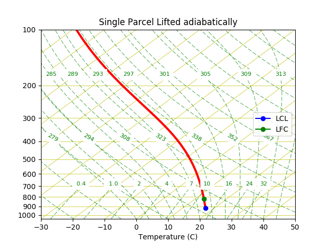
#Plot the parcel trajectory in the SkewT diagram

# First we lift the parcel adiabatically
initialLevel = myParcelAnalysis['initialLevel']

parcelTemperature = liftParcel(temperature[initialLevel],
                               pressure,
                               myParcelAnalysis['pressureAtLCL'],
                               initialLevel=initialLevel,
                               hPa=True,
                               celsius=True)


# Create a Figure Manager
mySkewT_Figure = figure()

# Add an Skew-T axes to the Figure
mySkewT_Axes = mySkewT_Figure.add_subplot(111, projection='skewx')

# Plot the parcel temperature
mySkewT_Axes.plot(parcelTemperature, pressure, linewidth=3, color='r' )

# Add a marker for the LCL and the LFC
mySkewT_Axes.plot(myParcelAnalysis['temperatureAtLCL'],
                  myParcelAnalysis['pressureAtLCL'],
                  marker='o', color='b' , label='LCL')
mySkewT_Axes.plot(myParcelAnalysis['temperatureAtLFC'],
                  myParcelAnalysis['pressureAtLFC'],
                  marker='o', color='g' , label='LFC')

# Add a legend
mySkewT_Axes.legend(loc='center right')

mySkewT_Axes.set_title("Single Parcel Lifted adiabatically")

mySkewT_Figure.show_plot()

In the next chapter, a more intensive use of the parcelAnalysis function is used to compute CAPE for a 3D domain from a WRF output file: WRF Output CAPE plot