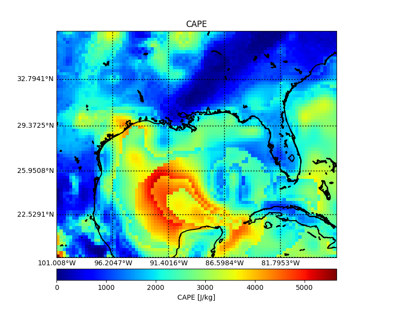
WRF Output CAPE plot

The SkewTplus.thermodynamics.parcelAnalysis() function allows to compute CAPE and CIN not only in a single vertical sounding, it also supports the computation over 3D domains (height, latitude or y , longitude or x) or 4D=(3D + time) ones (time, height, latitude or y, longitude or x].

Here is an example for computing CAPE from a WRF output file and plot the values as a color plot over a map:

from mpl_toolkits.basemap import Basemap
from netCDF4 import Dataset
import numpy

from SkewTplus.thermodynamics import parcelAnalysis
import matplotlib.pyplot as plt

#Load the WRF File
wrfOutputFile = Dataset("wrfOutputExample.nc")

theta = wrfOutputFile.variables["T"][:] + 300 # Potential temperature
pressure = wrfOutputFile.variables['P'][:] + wrfOutputFile.variables['PB'][:]

qvapor = wrfOutputFile.variables['QVAPOR'][:]

qvapor = numpy.ma.masked_where(qvapor <0.00002, qvapor)

T0 = 273.15
referencePressure = 100000.0  # [Pa]
epsilon = 0.622  # Rd / Rv

temperature = theta* numpy.power((pressure / referencePressure), 0.2854) - T0

vaporPressure = pressure * qvapor / (epsilon + qvapor)

dewPointTemperature = 243.5 / ((17.67 / numpy.log(vaporPressure * 0.01 / 6.112)) - 1.) #In celsius
dewPointTemperature = numpy.ma.masked_invalid(dewPointTemperature)


# Now we have the pressure, temperature and dew point temperature in the whole domain
# Compute the parcel analysis for each vertical column and each time
#
# fullFields =0 , only return CAPE and CIN
# Most Unstable  parcel : method=0
# Start looking for the most unstable parcel from the first level (initialLevel=0)
# Use at maximum 5 iterations in the bisection method to find the LCL
# Since the sounding temperature and pressure are expressed in Celsius and hPa
# we set the corresponding keywords
myParcelAnalysis = parcelAnalysis(pressure,
                                  temperature,
                                  dewPointTemperature,
                                  hPa=False,
                                  celsius=True,
                                  fullFields=0,
                                  method=0,
                                  initialLevel=0,
                                  tolerance=0.1,
                                  maxIterations=20)


## Create the Base Map for the CAPE color plot

# Read the temperature and pressure fields
lon = wrfOutputFile.variables["XLONG"][0, :, :]
lat = wrfOutputFile.variables["XLAT"][0, :, :]


#---Read lat,lon for plotting
lon = wrfOutputFile.variables["XLONG"][0, :, :]
lat = wrfOutputFile.variables["XLAT"][0, :, :]


# Define and plot the meridians and parallels
min_lat = numpy.amin(lat)
max_lat = numpy.amax(lat)
min_lon = numpy.amin(lon)
max_lon = numpy.amax(lon)

# Create the basemap object
myBaseMap = Basemap(projection="merc",
                    llcrnrlat=min_lat,
                    urcrnrlat=max_lat,
                    llcrnrlon=min_lon,
                    urcrnrlon=max_lon,
                    resolution='h')

# Create the figure and add axes
myFigure = plt.figure(figsize=(8,8))
myAxes = myFigure.add_axes([0.1,0.1,0.8,0.8])

# Make only 5 parallels and meridians
parallel_spacing = (max_lat - min_lat) / 5.0
merid_spacing = (max_lon - min_lon) / 5.0
parallels = numpy.arange(min_lat, max_lat, parallel_spacing)
meridians = numpy.arange(min_lon, max_lon, merid_spacing)

myBaseMap.drawcoastlines(linewidth=1.5)
myBaseMap.drawparallels(parallels,labels=[1,0,0,0],fontsize=10)
myBaseMap.drawmeridians(meridians,labels=[0,0,0,1],fontsize=10)

# Plot CAPE at time 0
CAPE = myParcelAnalysis['CAPE'][0,:]

myColorPlot = myBaseMap.pcolormesh(lon,lat, myParcelAnalysis['CAPE'][0,:],latlon=True, cmap='jet')

# Create the colorbar
cb = myBaseMap.colorbar(myColorPlot,"bottom", size="5%", pad="5%")
cb.set_label("CAPE [J/kg]")

# Set the plot title
myAxes.set_title("CAPE")

plt.show()